Version vom 7. Februar 2015, 17:39 Uhr

Abstract

NOTE: Everything under development here. Just showing ideas! :-)

The actual state of the robot can be described completely by:

• speed (m/s)
• direction (degree)
• position (x,y - meter)

All sensors (gyro, acceleration, compass, odometry, perimeter signal strength, GPS, ...) can deliver certain information about the robot's state. However, each sensor is noisy (added with errors). Sensor fusion is used to eliminate errors of each individual sensor. Each sensor gets a confidence weight that is automatically adjusted after reading the sensor by comparing its plausibility with the fusion result.

Sensor errors

• Odometry: accumulation error (e.g. 15cm per meter), update rate: 10-20 Hz
• Gyro: accumulation error (e.g. 1 degree per second), update rate: 10-20 Hz
• Compass: noise (e.g. 1 degree), update rate: 10-20 Hz
• GPS: noise (e.g. 2m), update rate: 1-5 Hz

Odometry sensor error

After a time, the odometry's error accumulates, and the course (Degree) and position (x/y) are getting unprecise.

Typical errors in outdoor condition (wet lawn, high slope):

• Distance: 20cm per meter
• Course: 10 degree per meter

The course can be permanently corrected by the compass sensor, the position by recalibration on the perimeter wire.

Sensor fusion

A Kalman or Extended Kalman Filter (EKF) filter can be used for sensor fusion.

Gyro         => Rotation speed delPhi   => 
Course(GPS)  => Course phiGPS           => Kalman =>  Course phi       =>                
Odometry     =>                                       Distance Sl, Sr  =>  Kalman  =>  Position x,y, Course phi

Note: This estimated position will need to be corrected by an absolute position estimation, e.g. perimeter field strength (and a particle filter).

Position recalibration

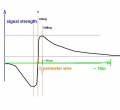
Because odometry error increases over time, the robot needs to periodically recalibrate its exact position (get the error to zero). This works by detecting its exact position on the perimeter wire (using cross correlation).

1. Learn mode: robot completely tracks perimeter wire once and saves course (degree) and distance (odometry ticks) in a list (perimeter tracking map).
2. Position detection: robot starts tracking the perimeter wire at arbitrary position until a high correlation with a subtrack of the perimeter tracking map is found. There it can stop tracking and knows its position on its perimeter tracking map.

Mapping and localization (SLAM)

The perimeter magnetic field could be used as input for a robot position estimation. However, as both the magnetic field map and the robot position on it is unknown, the algorithm needs to calculate both at the same time. Such algorithms are called 'Simultaneous Localization and Mapping' (SLAM).

Input to SLAM algorithm:

• control values (speed, steering)
• observation values (speed, heading, magnetic field strength)

Output from SLAM algorithm:

• magnetic field map (including perimeter border)
• robot position on that map (x,y,theta)

Example SLAM algorithms:

• Particle filter-based SLAM plus Rao-Blackwellization: model the robot’s path by sampling and compute the 'landmarks' given the poses

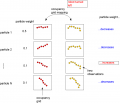
Example implementation: The idea is to use a particle filter that constantly generates a certain amount of 'guesses' (particles, e.g. N=50) where the robot can be (depending on the last position, control input, speed sensor and heading sensor measurements). Each 'particle' is evaluated by the perimeter field measurement...

• 

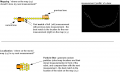
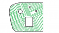
  strength precision is low in the center

• 

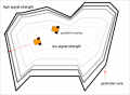
  same strenght values are located on rings

• 

  real measurements over a complete lawn

... and the particle 'weight' is adjusted based on that. Bad particles are replaced by new particles with new guesses near the good guesses. This constantly produces particles with high probability of the robot's location.

• 

  Perimeter magnetic field

• 

  SLAM (using magnetic field sensor)

• 

  SLAM (using classic LIDAR sensor)

• 

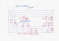
  SLAM (using 4 coils)

Videos: | Magnetic field localization using particle filter

Lane-by-lane mowing

In the lawn-by-lane mowing pattern, the robot uses a fixed course. When hitting an obstacle, the new course is added by 180 degree, so that the robot enters a new lane.

The robot always starts at the borders at an arbitrary choosen course, mowing lane by lane of a maximum length. The maximum length ensures that the odometry position error does not get too high. At the perimeter, the robot can reduce the error to zero again (one axis). The arbitrary starting course ensures that even small gaps on the lawn are mown completely after a 2nd mowing session (where the robot started at another arbitrary course).

• 

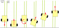
  Robot turns 180 degree and enters a new lane

• 

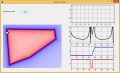
Simulation

Here's [1] a simulation of localization using odometry sensors.